Difference between revisions of "Guidelines for fishpasses numerical modelling"
Bendikhansen (talk | contribs) m (Text replacement - "{{Note|This technology has been developed in the FIThydro project! See Innovative technologies from FIThydro for a complete list.|reminder}} Innovative::developed in FIThydro" to "Innovative::developed in FIThydro|{{Note|This technology has been developed in the FIThydro project! See Innovative technologies from FIThydro for a complete list.|reminder}}]] ") |
Bendikhansen (talk | contribs) |
||
| (13 intermediate revisions by the same user not shown) | |||
| Line 1: | Line 1: | ||
| − | + | {{Note|This method has been developed in the FIThydro project! See [[Innovative technologies from FIThydro]] for a complete list.|reminder}} | |
| − | |||
=Quick summary= | =Quick summary= | ||
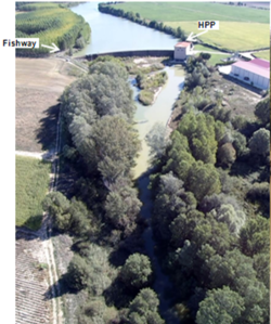
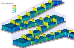
| − | [[file: | + | [[file:FPNM_guma.png|thumb|250px|Figure 1: Aerial view of the area downstream [[Guma and Vadocondes test cases|Guma HPP]].]] |
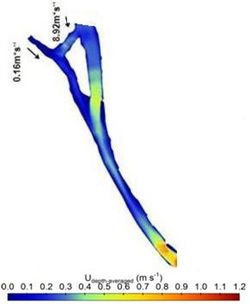
| − | + | [[file:FPNM_guma_2d.jpg|thumb|250px|Figure 2: Depth averaged velocity for the area downstream [[Guma and Vadocondes test cases|Guma HPP]] obtained with 2D numerical modelling.]] | |
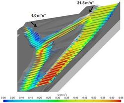
| + | [[file:FPNM_guma_3d.jpg|thumb|250px|Figure 3: Mean velocity magnitude in several cross sections for the area downstream [[Guma and Vadocondes test cases|Guma HPP]] obtained with 3D numerical modelling ]] | ||
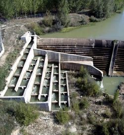
| + | [[file:FPNM_guma_aerial.jpg|thumb|250px|Figure 4: Aerial view of the [[Pool-type fishways|pool-type fishway]] at [[Guma and Vadocondes test cases|Guma HPP]] .]] | ||
| + | [[file:FPNM_isosurface.jpg|thumb|250px|Figure 5: Isosurface of the mean velocity in the fishway at [[Guma and Vadocondes test cases|Guma HPP]].]] | ||
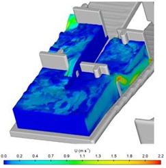
| + | [[file:FPNM_turning_pool.jpg|thumb|250px|Figure 6: Detailed results for a turning pool in the [[Pool-type fishways|pool-type fishway]] at [[Guma and Vadocondes test cases|Guma HPP]] obtained with 3D numerical modelling.]] | ||
| − | Date: | + | Date: 2020 |
| − | Developed by: | + | Developed by: Ana Quaresma (IST-ID), António Pinheiro (IST-ID) |
Type: [[:Category:Methods|Method]] | Type: [[:Category:Methods|Method]] | ||
=Introduction= | =Introduction= | ||
| + | Many efforts have been devoted to study, develop and optimize fishways design, construction and operation to improve their passability by fish, however fishway science, engineering and practice still remain imperfect (Silva et al., 2018). For a fishway to be fully functional its passability is vital. Nonetheless, its attraction ability is also critical. CFD is nowadays a major tool to study complex flow physics, and may be used to improve the design and operation of hydraulic structures, like fishways, reducing time and costs. The availability of different numerical methods options and its application in fishways calls for guidelines on its optimized use. To address this need, the Iberian test case of Guma HPP was chosen as a case study, along with previous work (Quaresma & Pinheiro, 2014;2015; Quaresma 2017; Quaresma et al. 2018), to develop guidelines for numerical modelling of fish passage facilities. 2D and 3D modelling of the attraction flow area at the fishway outflow of Guma HPP was performed to analyse hydrodynamic conditions to assess and improve fishway attractiveness. To analyse fishway operation, 3D modelling of the fishway under different flow regimes and operational constraints, such as clogged orifice or notch was conducted as well. From the numerical simulations carried out and from previous numerical modelling experience, a set of guidelines to be considered for similar numerical simulations of fish passage facilities was developed. | ||
=Application= | =Application= | ||
| + | Numerical modelling is an important tool to assess the flow patterns existing in a fishway and its downstream area and to assess the possible attractiveness improvements that riverbed morphology and change of HPP operation rules may bring. The flow patterns and possible recirculation zones are of course case specific and that means that each case must be analysed for different scenarios/discharges to identify the problematic areas and understand which morphologic or operation rules adaptations should be considered to improve the fishway attractiveness and passability. When compared to physical modelling or field tests, numerical modelling allows a less costly analysis of different scenarios/discharges and solutions, in shorter periods of time, before lab testing or construction. | ||
| + | |||
| + | From the numerical simulations carried out for Guma fishway, and for the downstream river reach, together with previous numerical modelling experience, it was possible to establish a set of recommendations/guidelines to be considered for similar numerical simulations: | ||
| + | |||
| + | ===Downstream reach modelling=== | ||
| + | * 1D modelling should be used for large-scale river channel hydraulics, since it gives a fast first assessment of flow velocities and depths. However, the flow features associated with streamlines curvature, confluences and flow obstructions (e.g. macro-roughness elements, boulders, and woody debris), cannot be adequately modelled. Whenever these situations occur, 2D or 3D numerical modelling should be applied. If the bathymetry of the downstream entrance of the migration device is smooth, 2D modelling is enough to validate the local velocities and the attraction flow pattern. If the river includes pronounced riverbed variations, confluences, and the near-bed hydraulic conditions are needed, 3D modelling should be used to better reproduce the region of interest. Depending on the area to simulate, it may be appropriate to establish a 1D or a 2D model in advance, whose results may be used as start conditions for the 3D models, to accelerate its convergence and reduce the 3D simulation time. | ||
| + | * When using 3D modelling, choosing the turbulence model is an important issue. If only discharge, flow depths and mean velocities are to be analysed, Reynolds-averaged Navier-Stokes (RANS) turbulence models may be used. If turbulence is important, Large eddy (LES) models more accurately reproduce the turbulence field (Quaresma, 2017). | ||
| + | * The bathymetric data resolution is vital to guarantee numerical modelling quality. 3D modelling requires more detailed topographical data than the 2D numerical model, to be effectively more accurate. For higher discharges, the wetted area is larger and, therefore, the topographic survey of the modelling domain should be larger, to capture all the flooded riverbed extent. | ||
| + | * The boundary conditions need to be carefully chosen and whenever possible boundaries should be located at gauging stations or where flow characteristics are better known or easily measured. When this is not possible, approximation using the normal depth may be used. However, care should be taken when using this strategy, by locating the boundary conditions as far as possible from the study area. | ||
| + | * In river channels, in HEC-RAS 2D model, to emulate steady-state conditions it is advisable to use inflow hydrographs that ramp up to the maximum discharge and maintain it for a duration enough to achieve steady state conditions, as rapid changes in the hydrodynamics of a model may result in unrealistic flow behaviour like extreme changes in depths and velocities. The duration of the ramp-up depends on the size and complexity of the domain and requires some sensitivity analysis from the user. | ||
| + | * Roughness estimation is an important issue for 2D depth-averaged models, and a careful calibration of this parameter is essential, given the higher sensitivity of 2D velocity predictions to roughness variation. Lane et al. (1999) addressed this problem. Knowledge of the site and photographs should be available to assist in roughness estimation. Although this is also important for 3D modelling, 3D models are less sensitive to roughness estimation. | ||
| + | |||
| + | ===Fishway modelling=== | ||
| + | * The accuracy of the fishway geometry is important to be able to simulate local conditions that determine fish behaviour. The fishway geometry should be adequately input in the model and reproduced by the numerical model to obtain an accurate numerical model. | ||
| + | * In vertical slot fishways with no macro-roughness elements or sills, the flow is almost 2D in the pool. Thus, 2D numerical modelling may be used. However, in pool-type fishways, flows through orifices and/or notches is clearly 3D. Hence, for these geometries, 3D modelling must be performed to accurately reproduce the flow field and correlate it with fish observations. 1D modelling may be carried just to use the results as start conditions for the 3D models to accelerate its convergence (Fuentes-Pérez et al, 2018b). | ||
| + | * To analyse a fishway hydrodynamics, the simulation time must always be considered when simulating long fishways. In fact, there may be no noticeable advantage in extending the simulation to the whole length of the fishway, since the flow characteristics will be repeated in subsequent pools once the uniform regime attains. In a sensitivity analysis, the user must figure out which number of pools needs to be considered to obtain representative results for the study case. | ||
| + | * Pools with different geometries, like resting pools, and larger pools that are usually installed in the fishway changes of direction, or the existence of pool geometry irregularities should be considered in the assessment of the number of pools to simulate. | ||
| + | * The boundary conditions need to be carefully chosen and whenever possible boundaries should be located where flow characteristics are better known or easily measured. In pool-type fishways, an approximation using the uniform flow design conditions may be used. However, a sufficient number of pools should be modelled, so that the results are not influenced by the boundary conditions and the simulation accuracy is not compromised. | ||
| + | * Non-uniform scenarios affect fishway hydrodynamics between different non-uniform situations, as well as, between pools. This variability is more challenging for fish to negotiate the fishway, since the hydraulic conditions change from pool to pool, which also changes the probability of successful negotiation of each cross-wall and may result in fish behaviour conditioning and modification, as already reported by Fuentes-Pérez et al. (2018a). Since these may naturally occur due to changes in the hydrological conditions over the year, fishways may need to be adapted, for example, with adaptable sills in the most downstream cross-walls or submerged pre-barrages downstream of the fishway as suggested by Fuentes-Pérez et al. (2016). | ||
| + | * Therefore, uniform and non-uniform regimes simulations must be carried out to assess the different conditions that fish will face when progressing upstream through the fishway. | ||
| + | |||
| + | ===Mesh resolution=== | ||
| + | * When using finite differences/volumes/elements methods, effective and efficient mesh development requires experience. Smaller cells are needed where flow hydrodynamics change more rapidly. Appropriate cells dimensions must be adapted to the bathymetry/geometry variation. The user should start with a coarser mesh and refine it until the results do not change significantly. Whenever possible, restart simulations based on coarser meshes results may be used. Restart simulations with grid overlay boundary conditions to refine and run smaller areas, might also be necessary. As restart simulations of the same domain with a finer mesh resolution allow for smaller computational times, and restart simulations for smaller domains allow for more detailed modelling of particular regions of interest. | ||
| + | * If no previous information is available, a good rule of thumb to pick the coarsest mesh to start the analysis is using 3 to 4 cells for resolving the flow, to test the model and the numerical options. However, usually 10 to 20 cells are needed to get a reasonably resolved velocity profile. | ||
| + | * To assess the mesh resolution, quality verification indexes should be used. For LES models, the LES_IQ index proposed by Celik et al. (2005) is recommended, whereas in RANS models, the Grid Convergence (GCI) method (Celik et al., 2008) should be used. It must, however, be emphasised that these indexes are verification indexes, which only assess mesh resolution quality. To assess model accuracy, a comparison with field/experimental data is always necessary, especially, if no previous applications of the used software to similar flow fields were performed. | ||
| + | |||
| + | ===Simulation time=== | ||
| + | * An important aspect for choosing the numerical model is the computational effort and the simulation time required, which are much larger in 3D modelling, compared to 2D modelling. So, one must ask if the additional parameters and flow information obtained with the 3D numerical modelling will be needed or used. For most fish species, no information on their behaviour in relation to e.g. 3D velocities, turbulence or eddies exists. Therefore, 3D modelling will not bring any substantial advantage, whereas it will increase the time needed to set-up the model and obtain results, compared to 2D modelling. | ||
| + | * To estimate the simulation time to reach steady state or to achieve a statistically stationary solution, and obtain converged time-averaged values, a good rule of thumb is considering 10 to 20 times the time required for the fluid to pass through the model domain. To estimate this time, whenever possible, 1D numerical modelling velocities may be used. | ||
| + | |||
| + | ===Model accuracy=== | ||
| + | * To assess model accuracy, a comparison with field/experimental data is still necessary, especially, whenever there are no previous applications of the used software to similar flow fields. Hydraulic data, like velocities and flow depths should be used to calibrate and validate the model, at least for one flow condition. Validation of the model guarantees its quality and helps in preventing and troubleshooting any problems, ensuring that the model adequately reproduces the modelled flow field within the desired tolerances. However, users should have experience with these type of simulations to be able to validate the numerical results and to interpret them from the fish preferences point of view. | ||
| + | * Differences between measurements and results from the numerical model may either be due to numerical simulations or measurements inaccuracy and scale issues. The physical limitations, as well as the measuring volume of the velocity measurement device used, must be considered together with possible numerical simulations limitations and the volume for which the model prediction is made. For instance, in Guma fishway, a larger difference was observed between the flow velocity measurement at the notches and the modelled value. The measurement was performed with a propeller, which measures the velocity component along its axis. Thus, a tilting of the instrument while measuring might also explain those differences. | ||
| + | |||
| + | ===Final remarks=== | ||
| + | * From the numerical simulations carried out, it was concluded that the increase of the attractiveness discharge does not necessarily imply better fishway performance because recirculation zones that may disorientate fish may form and hinder fishway attractiveness. Analysing the flow hydrodynamics in the downstream area of the fishway is thus essential. The flow patterns and possible recirculation zones are of course case specific, which implies case by case simulation and analysis. | ||
| + | * Due to the importance of the discharges coming from the HPP, attractiveness improvements must be analysed together with the operation rules of the powerhouse, and should serve as a basis to recommend operation rules adaption, if these prove to be necessary. Whenever information exists in literature for the target fish species, the modelled hydrodynamic parameters should be assessed and compared with these ones. | ||
| + | * Whenever information exists in literature regarding the target fish species preferences and capabilities, the modelled hydrodynamic parameters should be compared with those values (e.g. Quaresma et al., 2018) to assess the fishway hydrodynamics and evaluate its adequacy, and, if needed, to modify its design or retrofit existing ones. | ||
| + | * Finally, not only flow depths and velocities should be assessed, but turbulence parameters as well, since these are known to strongly influence fish behaviour (Cada et al., 1999; Liao, 2007; Silva et al., 2012; Tritico & Cotel, 2010) | ||
| + | . | ||
=Relevant mitigation measures and test cases= | =Relevant mitigation measures and test cases= | ||
| Line 21: | Line 65: | ||
=Relevant literature= | =Relevant literature= | ||
| + | |||
| + | *Cada G, Carlson T, Ferguson J, Richmond M, Sale M. 1999. Exploring the Role of Shear Stress and Severe Turbulence in Downstream Fish Passage. In Proceedings of the Waterpower Conference 1999; P. A. Brookshier (ed.) American Society of Civil Engineers (ASCE), Las Vegas, Nevada, United States 1999; p. 10. | ||
| + | *Celik IB, Cehreli ZN, Yavuz I. 2005. Index of resolution quality for large eddy simulations. J. Fluids Eng. 127 (5), 949–958. https://doi.org/10.1115/1.1990201 | ||
| + | *Celik IB, Ghia U, Roache PJ, Freitas CJ, Coleman H, Raad PE. 2008. Procedure for Estimation and Reporting of Uncertainty Due to Discretization in CFD Applications. J. Fluids Eng. 130(7), 078001-078001-4. doi: 10.1115/1.2960953 | ||
| + | *Fuentes-Pérez JF, Sanz-Ronda FJ, De Azagra AM, García-Vega A. 2016. Non-uniform hydraulic behavior of pool-weir fishways: A tool to optimize its design and performance. Ecological Engineering 86:5–12. doi: 10.1016/j.ecoleng.2015.10.021 | ||
| + | *Fuentes-Pérez JF, Eckert, M, Tuhtan JA, Ferreira MT, Kruusmaa M, Branco P. 2018a. Spatial preferences of Iberian barbel in a vertical slot fishway under variable hydrodynamic scenarios. Ecological Engineering 125:131-142. doi: 10.1016/j.ecoleng.2018.10.014 | ||
| + | *Fuentes-Pérez JF, Silva AT, Tuhtan JA, García-Vega A, Carbonell-Baeza R, Musall M, Kruusmaa M. 2018b. 3D modelling of non-uniform and turbulent flow in vertical slot fishways. Environmental Modelling & Software 99:156–169. https://doi.org/10.1016/jenvsoft.2017.09.011 | ||
| + | *Lane SN, Bradbrook KF, Richards KS, Biron PA, Roy AG. 1999. The application of computational fluid dynamics to natural river channels: three-dimensional versus two-dimensional approaches. Geomorphology 29:1-20. | ||
| + | *Liao JC. 2007. A review of fish swimming mechanics and behaviour in altered flows. Philosophical Transactions of the Royal Society B: Biological Sciences 362(1487): 1973-1993. | ||
| + | *Quaresma AL, Pinheiro AN. 2014. Analysis of flows in pool-type fishways using acoustic Doppler velocimetry (ADV) and computational fluid dynamics (CFD). Published in the 10th International Symposium on Ecohydraulics proceedings. Trondheim, Norway. | ||
| + | *Quaresma AL, Pinheiro AN. 2015. Is CFD an efficient tool to develop pool-type fishways? Fish Passage 2015 – International conference on river connectivity best practices and innovations. Groningen. Netherlands. | ||
| + | *Quaresma AL. 2017. Developing pool-type fishways based on experimental studies and numerical modelling. PhD Thesis, Instituto Superior Técnico, Universidade de Lisboa, Portugal. | ||
| + | *Quaresma AL, Romão F, Branco P, Ferreira MT & Pinheiro AN. 2018. Multi slot versus single slot pool-type fishways: a modelling approach to compare hydrodynamics. Ecological Engineering 122:197-206. doi:10.1016/j.ecoleng.2018.08.006 | ||
| + | *Silva AT, Katopodis C, Santos JM, Ferreira MT, Pinheiro AN. 2012. Cyprinid swimming behaviour in response to turbulent flow. Ecological Engineering 44:314–328. doi:10.1016/j.ecoleng.2012.04.015 | ||
| + | *Silva AT, Lucas MC, Castro-Santos T, Katopodis C, Baumgartner LJ, Thiem, JD, Aarestrup, K, Pompeu PS, O’Brien GC, Braun DC, Burnett NJ, Zhu DZ, Fjeldstad HP, Forseth T, Rajaratnam N, Williams JG & Cooke SJ. 2018. The future of fish passage science, engineering, and practice. Fish and Fisheries 19(2), 340–362. doi:10.1111/FAF.12258 | ||
| + | *Tritico HM, Cotel AJ. 2010. The effects of turbulent eddies on the stability and critical swimming speed of creek chub (Semotilus atromaculatus). Journal Experimental Biology 213:2284–2293. doi:10.1242/jeb.041806 | ||
| + | |||
| + | =Contact information:= | ||
| + | Ana Quaresma (IST-ID) | ||
| + | |||
| + | analopesquaresma@tecnico.ulisboa.pt | ||
| + | |||
| + | António Pinheiro (IST-ID) | ||
| + | |||
| + | antonio.pinheiro@tecnico.ulisboa.pt | ||
| + | |||
[[category:Methods]] [[Category:developed in FIThydro]] | [[category:Methods]] [[Category:developed in FIThydro]] | ||
Latest revision as of 08:47, 12 October 2020
Contents
Quick summary
Date: 2020
Developed by: Ana Quaresma (IST-ID), António Pinheiro (IST-ID)
Type: Method
Introduction
Many efforts have been devoted to study, develop and optimize fishways design, construction and operation to improve their passability by fish, however fishway science, engineering and practice still remain imperfect (Silva et al., 2018). For a fishway to be fully functional its passability is vital. Nonetheless, its attraction ability is also critical. CFD is nowadays a major tool to study complex flow physics, and may be used to improve the design and operation of hydraulic structures, like fishways, reducing time and costs. The availability of different numerical methods options and its application in fishways calls for guidelines on its optimized use. To address this need, the Iberian test case of Guma HPP was chosen as a case study, along with previous work (Quaresma & Pinheiro, 2014;2015; Quaresma 2017; Quaresma et al. 2018), to develop guidelines for numerical modelling of fish passage facilities. 2D and 3D modelling of the attraction flow area at the fishway outflow of Guma HPP was performed to analyse hydrodynamic conditions to assess and improve fishway attractiveness. To analyse fishway operation, 3D modelling of the fishway under different flow regimes and operational constraints, such as clogged orifice or notch was conducted as well. From the numerical simulations carried out and from previous numerical modelling experience, a set of guidelines to be considered for similar numerical simulations of fish passage facilities was developed.
Application
Numerical modelling is an important tool to assess the flow patterns existing in a fishway and its downstream area and to assess the possible attractiveness improvements that riverbed morphology and change of HPP operation rules may bring. The flow patterns and possible recirculation zones are of course case specific and that means that each case must be analysed for different scenarios/discharges to identify the problematic areas and understand which morphologic or operation rules adaptations should be considered to improve the fishway attractiveness and passability. When compared to physical modelling or field tests, numerical modelling allows a less costly analysis of different scenarios/discharges and solutions, in shorter periods of time, before lab testing or construction.
From the numerical simulations carried out for Guma fishway, and for the downstream river reach, together with previous numerical modelling experience, it was possible to establish a set of recommendations/guidelines to be considered for similar numerical simulations:
Downstream reach modelling
- 1D modelling should be used for large-scale river channel hydraulics, since it gives a fast first assessment of flow velocities and depths. However, the flow features associated with streamlines curvature, confluences and flow obstructions (e.g. macro-roughness elements, boulders, and woody debris), cannot be adequately modelled. Whenever these situations occur, 2D or 3D numerical modelling should be applied. If the bathymetry of the downstream entrance of the migration device is smooth, 2D modelling is enough to validate the local velocities and the attraction flow pattern. If the river includes pronounced riverbed variations, confluences, and the near-bed hydraulic conditions are needed, 3D modelling should be used to better reproduce the region of interest. Depending on the area to simulate, it may be appropriate to establish a 1D or a 2D model in advance, whose results may be used as start conditions for the 3D models, to accelerate its convergence and reduce the 3D simulation time.
- When using 3D modelling, choosing the turbulence model is an important issue. If only discharge, flow depths and mean velocities are to be analysed, Reynolds-averaged Navier-Stokes (RANS) turbulence models may be used. If turbulence is important, Large eddy (LES) models more accurately reproduce the turbulence field (Quaresma, 2017).
- The bathymetric data resolution is vital to guarantee numerical modelling quality. 3D modelling requires more detailed topographical data than the 2D numerical model, to be effectively more accurate. For higher discharges, the wetted area is larger and, therefore, the topographic survey of the modelling domain should be larger, to capture all the flooded riverbed extent.
- The boundary conditions need to be carefully chosen and whenever possible boundaries should be located at gauging stations or where flow characteristics are better known or easily measured. When this is not possible, approximation using the normal depth may be used. However, care should be taken when using this strategy, by locating the boundary conditions as far as possible from the study area.
- In river channels, in HEC-RAS 2D model, to emulate steady-state conditions it is advisable to use inflow hydrographs that ramp up to the maximum discharge and maintain it for a duration enough to achieve steady state conditions, as rapid changes in the hydrodynamics of a model may result in unrealistic flow behaviour like extreme changes in depths and velocities. The duration of the ramp-up depends on the size and complexity of the domain and requires some sensitivity analysis from the user.
- Roughness estimation is an important issue for 2D depth-averaged models, and a careful calibration of this parameter is essential, given the higher sensitivity of 2D velocity predictions to roughness variation. Lane et al. (1999) addressed this problem. Knowledge of the site and photographs should be available to assist in roughness estimation. Although this is also important for 3D modelling, 3D models are less sensitive to roughness estimation.
Fishway modelling
- The accuracy of the fishway geometry is important to be able to simulate local conditions that determine fish behaviour. The fishway geometry should be adequately input in the model and reproduced by the numerical model to obtain an accurate numerical model.
- In vertical slot fishways with no macro-roughness elements or sills, the flow is almost 2D in the pool. Thus, 2D numerical modelling may be used. However, in pool-type fishways, flows through orifices and/or notches is clearly 3D. Hence, for these geometries, 3D modelling must be performed to accurately reproduce the flow field and correlate it with fish observations. 1D modelling may be carried just to use the results as start conditions for the 3D models to accelerate its convergence (Fuentes-Pérez et al, 2018b).
- To analyse a fishway hydrodynamics, the simulation time must always be considered when simulating long fishways. In fact, there may be no noticeable advantage in extending the simulation to the whole length of the fishway, since the flow characteristics will be repeated in subsequent pools once the uniform regime attains. In a sensitivity analysis, the user must figure out which number of pools needs to be considered to obtain representative results for the study case.
- Pools with different geometries, like resting pools, and larger pools that are usually installed in the fishway changes of direction, or the existence of pool geometry irregularities should be considered in the assessment of the number of pools to simulate.
- The boundary conditions need to be carefully chosen and whenever possible boundaries should be located where flow characteristics are better known or easily measured. In pool-type fishways, an approximation using the uniform flow design conditions may be used. However, a sufficient number of pools should be modelled, so that the results are not influenced by the boundary conditions and the simulation accuracy is not compromised.
- Non-uniform scenarios affect fishway hydrodynamics between different non-uniform situations, as well as, between pools. This variability is more challenging for fish to negotiate the fishway, since the hydraulic conditions change from pool to pool, which also changes the probability of successful negotiation of each cross-wall and may result in fish behaviour conditioning and modification, as already reported by Fuentes-Pérez et al. (2018a). Since these may naturally occur due to changes in the hydrological conditions over the year, fishways may need to be adapted, for example, with adaptable sills in the most downstream cross-walls or submerged pre-barrages downstream of the fishway as suggested by Fuentes-Pérez et al. (2016).
- Therefore, uniform and non-uniform regimes simulations must be carried out to assess the different conditions that fish will face when progressing upstream through the fishway.
Mesh resolution
- When using finite differences/volumes/elements methods, effective and efficient mesh development requires experience. Smaller cells are needed where flow hydrodynamics change more rapidly. Appropriate cells dimensions must be adapted to the bathymetry/geometry variation. The user should start with a coarser mesh and refine it until the results do not change significantly. Whenever possible, restart simulations based on coarser meshes results may be used. Restart simulations with grid overlay boundary conditions to refine and run smaller areas, might also be necessary. As restart simulations of the same domain with a finer mesh resolution allow for smaller computational times, and restart simulations for smaller domains allow for more detailed modelling of particular regions of interest.
- If no previous information is available, a good rule of thumb to pick the coarsest mesh to start the analysis is using 3 to 4 cells for resolving the flow, to test the model and the numerical options. However, usually 10 to 20 cells are needed to get a reasonably resolved velocity profile.
- To assess the mesh resolution, quality verification indexes should be used. For LES models, the LES_IQ index proposed by Celik et al. (2005) is recommended, whereas in RANS models, the Grid Convergence (GCI) method (Celik et al., 2008) should be used. It must, however, be emphasised that these indexes are verification indexes, which only assess mesh resolution quality. To assess model accuracy, a comparison with field/experimental data is always necessary, especially, if no previous applications of the used software to similar flow fields were performed.
Simulation time
- An important aspect for choosing the numerical model is the computational effort and the simulation time required, which are much larger in 3D modelling, compared to 2D modelling. So, one must ask if the additional parameters and flow information obtained with the 3D numerical modelling will be needed or used. For most fish species, no information on their behaviour in relation to e.g. 3D velocities, turbulence or eddies exists. Therefore, 3D modelling will not bring any substantial advantage, whereas it will increase the time needed to set-up the model and obtain results, compared to 2D modelling.
- To estimate the simulation time to reach steady state or to achieve a statistically stationary solution, and obtain converged time-averaged values, a good rule of thumb is considering 10 to 20 times the time required for the fluid to pass through the model domain. To estimate this time, whenever possible, 1D numerical modelling velocities may be used.
Model accuracy
- To assess model accuracy, a comparison with field/experimental data is still necessary, especially, whenever there are no previous applications of the used software to similar flow fields. Hydraulic data, like velocities and flow depths should be used to calibrate and validate the model, at least for one flow condition. Validation of the model guarantees its quality and helps in preventing and troubleshooting any problems, ensuring that the model adequately reproduces the modelled flow field within the desired tolerances. However, users should have experience with these type of simulations to be able to validate the numerical results and to interpret them from the fish preferences point of view.
- Differences between measurements and results from the numerical model may either be due to numerical simulations or measurements inaccuracy and scale issues. The physical limitations, as well as the measuring volume of the velocity measurement device used, must be considered together with possible numerical simulations limitations and the volume for which the model prediction is made. For instance, in Guma fishway, a larger difference was observed between the flow velocity measurement at the notches and the modelled value. The measurement was performed with a propeller, which measures the velocity component along its axis. Thus, a tilting of the instrument while measuring might also explain those differences.
Final remarks
- From the numerical simulations carried out, it was concluded that the increase of the attractiveness discharge does not necessarily imply better fishway performance because recirculation zones that may disorientate fish may form and hinder fishway attractiveness. Analysing the flow hydrodynamics in the downstream area of the fishway is thus essential. The flow patterns and possible recirculation zones are of course case specific, which implies case by case simulation and analysis.
- Due to the importance of the discharges coming from the HPP, attractiveness improvements must be analysed together with the operation rules of the powerhouse, and should serve as a basis to recommend operation rules adaption, if these prove to be necessary. Whenever information exists in literature for the target fish species, the modelled hydrodynamic parameters should be assessed and compared with these ones.
- Whenever information exists in literature regarding the target fish species preferences and capabilities, the modelled hydrodynamic parameters should be compared with those values (e.g. Quaresma et al., 2018) to assess the fishway hydrodynamics and evaluate its adequacy, and, if needed, to modify its design or retrofit existing ones.
- Finally, not only flow depths and velocities should be assessed, but turbulence parameters as well, since these are known to strongly influence fish behaviour (Cada et al., 1999; Liao, 2007; Silva et al., 2012; Tritico & Cotel, 2010)
.
Relevant mitigation measures and test cases
Other information
Relevant literature
- Cada G, Carlson T, Ferguson J, Richmond M, Sale M. 1999. Exploring the Role of Shear Stress and Severe Turbulence in Downstream Fish Passage. In Proceedings of the Waterpower Conference 1999; P. A. Brookshier (ed.) American Society of Civil Engineers (ASCE), Las Vegas, Nevada, United States 1999; p. 10.
- Celik IB, Cehreli ZN, Yavuz I. 2005. Index of resolution quality for large eddy simulations. J. Fluids Eng. 127 (5), 949–958. https://doi.org/10.1115/1.1990201
- Celik IB, Ghia U, Roache PJ, Freitas CJ, Coleman H, Raad PE. 2008. Procedure for Estimation and Reporting of Uncertainty Due to Discretization in CFD Applications. J. Fluids Eng. 130(7), 078001-078001-4. doi: 10.1115/1.2960953
- Fuentes-Pérez JF, Sanz-Ronda FJ, De Azagra AM, García-Vega A. 2016. Non-uniform hydraulic behavior of pool-weir fishways: A tool to optimize its design and performance. Ecological Engineering 86:5–12. doi: 10.1016/j.ecoleng.2015.10.021
- Fuentes-Pérez JF, Eckert, M, Tuhtan JA, Ferreira MT, Kruusmaa M, Branco P. 2018a. Spatial preferences of Iberian barbel in a vertical slot fishway under variable hydrodynamic scenarios. Ecological Engineering 125:131-142. doi: 10.1016/j.ecoleng.2018.10.014
- Fuentes-Pérez JF, Silva AT, Tuhtan JA, García-Vega A, Carbonell-Baeza R, Musall M, Kruusmaa M. 2018b. 3D modelling of non-uniform and turbulent flow in vertical slot fishways. Environmental Modelling & Software 99:156–169. https://doi.org/10.1016/jenvsoft.2017.09.011
- Lane SN, Bradbrook KF, Richards KS, Biron PA, Roy AG. 1999. The application of computational fluid dynamics to natural river channels: three-dimensional versus two-dimensional approaches. Geomorphology 29:1-20.
- Liao JC. 2007. A review of fish swimming mechanics and behaviour in altered flows. Philosophical Transactions of the Royal Society B: Biological Sciences 362(1487): 1973-1993.
- Quaresma AL, Pinheiro AN. 2014. Analysis of flows in pool-type fishways using acoustic Doppler velocimetry (ADV) and computational fluid dynamics (CFD). Published in the 10th International Symposium on Ecohydraulics proceedings. Trondheim, Norway.
- Quaresma AL, Pinheiro AN. 2015. Is CFD an efficient tool to develop pool-type fishways? Fish Passage 2015 – International conference on river connectivity best practices and innovations. Groningen. Netherlands.
- Quaresma AL. 2017. Developing pool-type fishways based on experimental studies and numerical modelling. PhD Thesis, Instituto Superior Técnico, Universidade de Lisboa, Portugal.
- Quaresma AL, Romão F, Branco P, Ferreira MT & Pinheiro AN. 2018. Multi slot versus single slot pool-type fishways: a modelling approach to compare hydrodynamics. Ecological Engineering 122:197-206. doi:10.1016/j.ecoleng.2018.08.006
- Silva AT, Katopodis C, Santos JM, Ferreira MT, Pinheiro AN. 2012. Cyprinid swimming behaviour in response to turbulent flow. Ecological Engineering 44:314–328. doi:10.1016/j.ecoleng.2012.04.015
- Silva AT, Lucas MC, Castro-Santos T, Katopodis C, Baumgartner LJ, Thiem, JD, Aarestrup, K, Pompeu PS, O’Brien GC, Braun DC, Burnett NJ, Zhu DZ, Fjeldstad HP, Forseth T, Rajaratnam N, Williams JG & Cooke SJ. 2018. The future of fish passage science, engineering, and practice. Fish and Fisheries 19(2), 340–362. doi:10.1111/FAF.12258
- Tritico HM, Cotel AJ. 2010. The effects of turbulent eddies on the stability and critical swimming speed of creek chub (Semotilus atromaculatus). Journal Experimental Biology 213:2284–2293. doi:10.1242/jeb.041806
Contact information:
Ana Quaresma (IST-ID)
analopesquaresma@tecnico.ulisboa.pt
António Pinheiro (IST-ID)
antonio.pinheiro@tecnico.ulisboa.pt
